lmSubsets: Exact variable-subset selection in linear regression
Citation
Hofmann M, Gatu C, Kontoghiorghes EJ, Colubi A, Zeileis A (2020). “lmSubsets: Exact Variable-Subset Selection in Linear Regression for R.” Journal of Statistical Software, 93(3), 1-21. doi:10.18637/jss.v093.i03
Abstract
An R package for computing the all-subsets regression problem is presented. The proposed algorithms are based on computational strategies recently developed. A novel algorithm for the best-subset regression problem selects subset models based on a predetermined criterion. The package user can choose from exact and from approximation algorithms. The core of the package is written in C++ and provides an efficient implementation of all the underlying numerical computations. A case study and benchmark results illustrate the usage and the computational efficiency of the package.
Software
https://CRAN.R-project.org/package=lmSubsets
Illustration: Variable selection in weather forecasting
Advances in numerical weather prediction (NWP) have played an important role in the increase of weather forecast skill over the past decades. Numerical models simulate physical systems that operate at a large, typically global, scale. The horizontal (spatial) resolution is limited by the computational power available today and hence, typically, the NWP outputs are post-processed to correct for local and unresolved effects in order to obtain forecasts for specific locations. So-called model output statistics (MOS) develops a regression relationship based on past meteorological observations of the variable to be predicted and forecasted NWP quantities at a certain lead time. Variable-subset selection is often employed to determine which NWP outputs should be included in the regression model for a specific location.
Here, the lmSubsets package is used to build a MOS regression model predicting temperature at Innsbruck Airport, Austria, based on data from the Global Ensemble Forecast System. The data frame IbkTemperature contains 1824 daily cases for 42 variables: the temperature at Innsbruck Airport (observed), 36 NWP outputs (forecasted), and 5 deterministic time trend/season patterns. The NWP variables include quantities pertaining to temperature (e.g., 2-meter above ground, minimum, maximum, soil), precipitation, wind, and fluxes, among others.
First, package and data are loaded and the few missing values are omitted for simplicity.
library("lmSubsets")
data("IbkTemperature", package = "lmSubsets")
IbkTemperature <- na.omit(IbkTemperature)
A simple output model for the observed temperature (temp) is constructed, which will serve as the reference model. It consists of the 2-meter temperature NWP forecast (t2m), a linear trend component (time), as well as seasonal components with annual (sin, cos) and bi-annual (sin2, cos2) harmonic patterns.
MOS0 <- lm(temp ~ t2m + time + sin + cos + sin2 + cos2,
  data = IbkTemperature)
When looking at summary(MOS0) or the coefficient table below, it can be observed that despite the inclusion of the NWP variable t2m, the coefficients for the deterministic components remain significant, which indicates that the seasonal temperature fluctuations are not fully resolved by the numerical model.
| MOS0 | MOS1 | MOS2 | ||||
| (Intercept) | -345.252 ** | (109.212) | -666.584 *** | (95.349) | -661.700 *** | (95.225) |
| t2m | 0.318 *** | (0.016) | 0.055 | (0.029) | ||
| time | 0.132 * | (0.054) | 0.149 ** | (0.047) | 0.147 ** | (0.047) |
| sin | -1.234 *** | (0.126) | 0.522 *** | (0.147) | 0.811 *** | (0.120) |
| cos | -6.329 *** | (0.164) | -0.812 ** | (0.273) | ||
| sin2 | 0.240 * | (0.110) | -0.794 *** | (0.119) | -0.870 *** | (0.118) |
| cos2 | -0.332 ** | (0.109) | -1.067 *** | (0.101) | -1.128 *** | (0.097) |
| sshnf | 0.016 *** | (0.004) | 0.018 *** | (0.004) | ||
| vsmc | 20.200 *** | (3.115) | 20.181 *** | (3.106) | ||
| tmax2m | 0.145 *** | (0.037) | 0.181 *** | (0.023) | ||
| st | 1.077 *** | (0.051) | 1.142 *** | (0.043) | ||
| wr | 0.450 *** | (0.109) | 0.505 *** | (0.103) | ||
| t2pvu | 0.064 *** | (0.011) | 0.149 *** | (0.028) | ||
| mslp | -0.000 *** | (0.000) | ||||
| p2pvu | -0.000 ** | (0.000) | ||||
| AIC | 9493.602 | 8954.907 | 8948.182 | |||
| BIC | 9537.650 | 9031.992 | 9025.267 | |||
| RSS | 19506.469 | 14411.122 | 14357.943 | |||
| Sigma | 3.281 | 2.825 | 2.820 | |||
| R-squared | 0.803 | 0.854 | 0.855 | |||
| *** p < 0.001; ** p < 0.01; * p < 0.05. | ||||||
Next, the reference model is extended with selected regressors taken from the remaining 35 NWP variables.
MOS1_best <- lmSelect(temp ~ ., data = IbkTemperature,
  include = c("t2m", "time", "sin", "cos", "sin2", "cos2"),
  penalty = "BIC", nbest = 20)
MOS1 <- refit(MOS1_best)
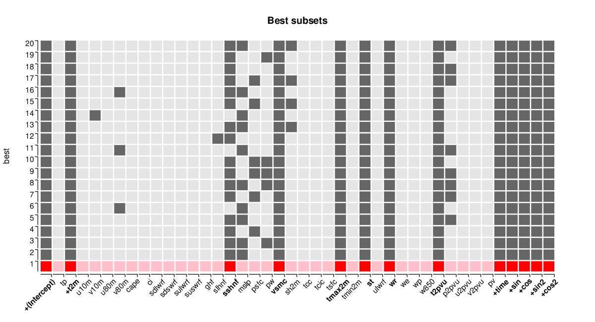
Best-subset regression with respect to the BIC criterion is employed to determine pertinent veriables in addition to the regressors already used in MOS0. The 20 best submodels are computed and the selected variables can be visualized by image(MOS1_best, hilite = 1) (see below) while the corresponding BIC values can be visualized by plot(MOS1_best). All in all, these 20 best models are very similar with only a few variables switching between being included and excluded. Using the refit() method the best submodel can be extracted and fitted via lm(). Summary statistics are shown in the table above. Overall, the model MOS1 improves the model fit considerably compared to the basic MOS0 model.
Finally, an all-subsets regression is conducted instead of the cheaper best-subsets regression. It considers all 41 variables without any restrictions to determine what is the best model in terms of BIC that could be found for this data set.
MOS2_all <- lmSubsets(temp ~ ., data = IbkTemperature)
MOS2 <- refit(lmSelect(MOS2_all, penalty = "BIC"))
Again, the best model is refitted with lm() to facilitate further inspections, see above for the summary table.
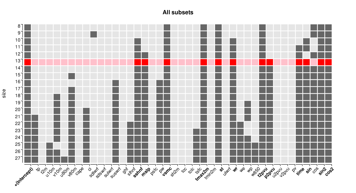
The best-BIC models MOS1 and MOS2 both have 13 regressors. The deterministic trend and all but one of the harmonic seasonal components are retained in MOS2 even though they are not forced into the model (as in MOS1). In addition, MOS1 and MOS2 share six NWP outputs relating to temperature (tmax2m, st, t2pvu), pressure (mslp, p2pvu), hydrology (vsmc, wr), and heat flux (sshnf). However, and most remarkably, MOS1 does not include the direct 2-meter temperature output from the NWP model (t2m). In fact, t2m is not included by any of the 20 submodels (sizes 8 to 27) shown by image(MOS2_all, size = 8:27, hilite = 1, hilite_penalty = "BIC") whereas the temperature quantities tmax2m, st, t2pvu are included by all. (Additionally, plot(MOS2_all) would show the associated BIC and residual sum of squares across the different model sizes.) The summary statistics reveal that both MOS1 and MOS2 significantly improve over the simple reference model MOS0, with MOS2 being only slightly better than MOS1.

