Structural equation model trees with partykit and lavaan
Motivation
Structural equation models (SEMs) are a popular class of models, especially in the social sciences, to model correlations and dependencies in multivariate data, often involving latent variables. To account for individual heterogeneities in the SEM parameters sometimes finite-mixture models are used, in particular when there are no covariates available to explain the source of the heterogeneity. More recently, starting from the work of Brandmaier et al. (2013, Psychological Methods, doi:10.1037/a0030001) tree-based modeling of SEMs has also been receiving increasing interest in the literature. Based on available covariates SEM trees can capture the heterogeneity by recursively partitioning the data into subgroups. Brandmaier et al. also provide an R implementation for their algorithm in their semtree package available from CRAN.
Their original SEM tree algorithm relied on selecting the variables for recursive partitioning based on likelihood ratio tests along with somewhat ad hoc adjustments. Recently, the group around Brandmaier proposed to use score-based tests instead that account more formally for selecting the maximal statistic across a range of possible split points (see Arnold et al. 2020, PsyArXiv Preprints, doi:10.31234/osf.io/65bxv). They show that this not only improves the accuracy of the method but can also greatly alleviate the computational burden.
The score-based tests draw on the work started by us in Merkle & Zeileis (2013, Psychometrika, doi:10.1007/s11336-012-9302-4) which in fact had already long been available in a general model-based tree algorithm (called MOB for short), proposed by us in Zeileis et al. (2008, Journal of Computational and Graphical Statistics, doi:10.1198/106186008X319331) and available in the R package partykit (and party before that).
In this blog post I show how the general mob() function from partykit can be easily coupled with the lavaan package (Rosseel 2012, Journal of Statistical Software, doi:10.18637/jss.v048.i02) as an alternative approach to fitting SEM trees.
MOB: Model-based recursive partitioning
MOB is a very broad tree algorithm that can capture subgroups in general parametric models (e.g., probability distributions, regression models, measurement models, etc.). While it can be applied to M-type estimators in general, it is probably easiest to outline the algorithm for maximum likelihood models. The algorithm assumes that there is some data of interest along with a suitable model that can fit the data, at least locally in subgroups. And additionally there are further covariates that can be used for splitting the data to find these subgroups. It proceeds in the following steps.
- Estimate the model parameters by maximum likelihood for the observations in the current subsample.
- Test for associations (or instabilities) of the corresponding model scores and each of the covariates available for splitting.
- Split the sample along the covariate with the strongest association or instability. Choose the breakpoint with the highest improvement in the log-likelihood.
- Repeat steps 1-3 recursively in the subsamples until these become too small or there is no significant association/instability (or some other stopping criterion is reached).
- Optionally: Reduce size of the tree by pruning branches of splits that do not improve the model fit sufficiently (e.g., based on information criteria).
The mob() function in partykit implements this general algorithm and allows to plug in different model-fitting functions, provided they allow to extract the estimated parameters, the maximized log-likelihood, and the corresponding matrix of score (or gradient) contributions for each observation. The details are described in a vignette within the package: Parties, Models, Mobsters: A New Implementation of Model-Based Recursive Partitioning in R.
A SEM mobster using lavaan
As the lavaan package readily provides the quantities that MOB needs as input we can easily set up a “mobster” function for SEMs. The lavaan_fit() function below takes a lavaan model definition and returns the actual fitting function with the interface as required by mob():
lavaan_fit <- function(model) {
  function(y, x = NULL, start = NULL, weights = NULL, offset = NULL, ..., estfun = FALSE, object = FALSE) {
    sem <- lavaan::lavaan(model = model, data = y, start = start)
    list(
      coefficients = stats4::coef(sem),
      objfun = -as.numeric(stats4::logLik(sem)),
      estfun = if(estfun) sandwich::estfun(sem) else NULL,
      object = if(object) sem else NULL
    )
  }
}
The fitting function just calls lavaan() using the model, the data y, and optionally the start-ing values, ignoring other arguments that mob() could handle. It then extracts the parameters coef(), the log-likelihood logLik(), and the score matrix estfun() using the generic functions from the corresponding packages and returns them in a list.
Illustration: Linear growth curve model tree
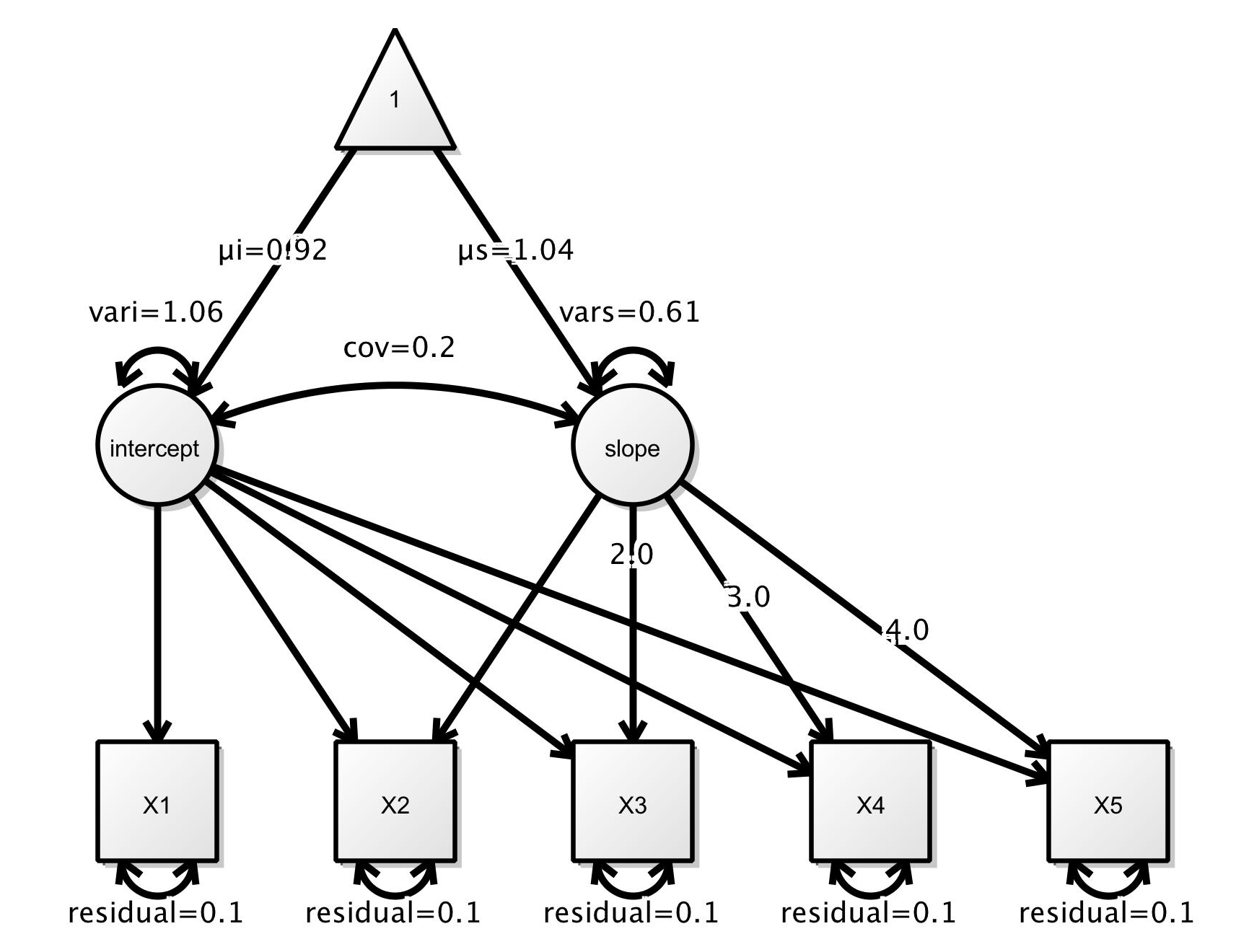
To illustrate fitting SEM trees with partykit and lavaan, we consider the example from the Using lavaan with semtree tutorial provided by Brandmaier et al.. It is a linear growth curve model for data measured at five time points: X1, X2, X3, X4, and X5. The main parameters of interest are the intercept and the slope of the growth curves while accounting for random variations and correlations among the involved variables according to this SEM. In lavaan notation:
growth_curve_model <- '
  inter =~ 1*X1 + 1*X2 + 1*X3 + 1*X4 + 1*X5;
  slope =~ 0*X1 + 1*X2 + 2*X3 + 3*X4 + 4*X5;
  inter ~~ vari*inter; inter ~ meani*1;
  slope ~~ vars*slope; slope ~ means*1;
  inter ~~ cov*slope;
  X1 ~~ residual*X1; X1 ~ 0*1;
  X2 ~~ residual*X2; X2 ~ 0*1;
  X3 ~~ residual*X3; X3 ~ 0*1;
  X4 ~~ residual*X4; X4 ~ 0*1;
  X5 ~~ residual*X5; X5 ~ 0*1;
'
The model can also be visualized using the following graphic taken from the tutorial:
In addition to the measurements at the five time points, the data set example1.txt provides three covariates (agegroup, training, and noise) that can be used to capture individual difference in the model parameters. The data can be read and transformed to appropriate classes by:
ex1 <- data.frame(read.csv(
  "https://brandmaier.de/semtree/wp-content/uploads/downloads/2012/07/example1.txt",
  sep = "\t"))
ex1 <- transform(ex1,
  agegroup = factor(agegroup),
  training = factor(training),
  noise = factor(noise))
Fitting the SEM tree
Given the data, model, and mobster function are available, it is easy to fit the MOB tree with SEMs in every node of the tree. The five measurements are the dependent variables (y) that need to be passed to the model as a "data.frame", the three covariates are the explanatory variables:
library("partykit")
tr <- mob(X1 + X2 + X3 + X4 + X5 ~ agegroup + training + noise, data = ex1,
  fit = lavaan_fit(growth_curve_model),
  control = mob_control(ytype = "data.frame"))
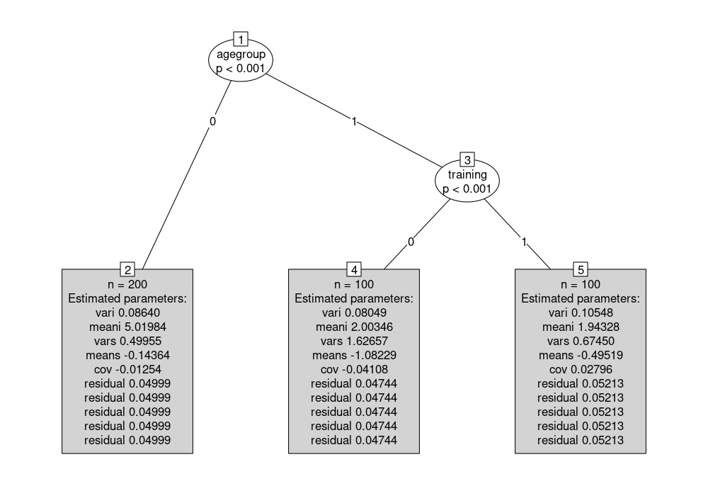
The resulting tree tr correctly detects the three subgroups that were simulated for the data by Brandmaier et al.. It can be visualized (with somewhat larger terminal nodes, all dropped to the bottom of the display):
plot(tr, drop = TRUE, tnex = 2)
The parameter estimates can also be extracted by coef(tr):
t(coef(tr))
##               2      4      5
## vari      0.086  0.080  0.105
## meani     5.020  2.003  1.943
## vars      0.500  1.627  0.675
## means    -0.144 -1.082 -0.495
## cov      -0.013 -0.041  0.028
## residual  0.050  0.047  0.052
## residual  0.050  0.047  0.052
## residual  0.050  0.047  0.052
## residual  0.050  0.047  0.052
## residual  0.050  0.047  0.052
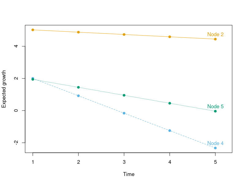
The main parameters of interest are meani, the mean intercept, and means, the mean slope that both vary across the subgroups defined by agegroup and training: In node 2 the intercept is about 5 while in nodes 4 and 5 it is around 2. The slope is almost zero in node 2, about -1 in node 4, and about -0.5 in node 5. The residual variance is restricted to be constant across the five time points and hence repeated in the output.
Further displays
By extracting the node-specific meani and means parameters, the expected growth can also be visualized in the following way:
gr <- coef(tr)[, "meani"] + outer(coef(tr)[, "means"], 0:4)
cl <- palette.colors(4, "Okabe-Ito")[-1]
matplot(t(gr), type = "o", pch = 19, col = cl,
  ylab = "Expected growth", xlab = "Time", xlim = c(1, 5.2))
text(5, gr[, 5], paste("Node", rownames(gr)), col = cl, pos = 3)
Finally, using a custom printing function that only shows the subgroup size and the first six parameters, the tree can be nicely printed as:
node_format <- function(node) {
  c("",
    sprintf("n = %s", node$nobs),
    capture.output(print(cbind(node$coefficients[1:6]), digits = 2L))[-1L])
}
print(tr, FUN = node_format)
## Model-based recursive partitioning (lavaan_fit(growth_curve_model))
##
## Model formula:
## X1 + X2 + X3 + X4 + X5 ~ agegroup + training + noise
##
## Fitted party:
## [1] root
## |   [2] agegroup in 0
## |       n = 200
## |       vari      0.086
## |       meani     5.020
## |       vars      0.500
## |       means    -0.144
## |       cov      -0.013
## |       residual  0.050
## |   [3] agegroup in 1
## |   |   [4] training in 0
## |   |       n = 100
## |   |       vari      0.080
## |   |       meani     2.003
## |   |       vars      1.627
## |   |       means    -1.082
## |   |       cov      -0.041
## |   |       residual  0.047
## |   |   [5] training in 1
## |   |       n = 100
## |   |       vari      0.105
## |   |       meani     1.943
## |   |       vars      0.675
## |   |       means    -0.495
## |   |       cov       0.028
## |   |       residual  0.052
##
## Number of inner nodes:    2
## Number of terminal nodes: 3
## Number of parameters per node: 10
## Objective function: 1330.735
Concluding remarks
The main purpose of this blog post was to show that it is relatively simple to fit model-based trees with custom models using the general mob() infrastructure from the partykit package. Specifically, lavaan makes it easy to fit SEM trees as the lavaan package readily provides all necessary components. As I had provided this as feedback to Arnold et al. and encouraged them to drill a bit deeper to better understand the differences between their adapted SEM tree algorithm and MOB, I thought I should share the code as it might be useful to others as well.
One important difference between the new SEM tree algorithm and the current MOB implementation is the determination of the best split point. The new SEM tree also uses the scores for this while MOB is based on the log-likelihood in the subgroups and hence is slower searching splits in numeric covariates with many possible split points. While we also had experimented with score-based split point estimation in party this has never been released and is currently not available in partykit. However, we are working on making the split point selection more flexible in partykit.
Of course, fitting the tree model is actually just the first step in an analysis of subgroups in a SEM. The subsequent steps for analyzing and interpreting the resulting tree model are at least as important. The work bei Brandmaier and his co-authors and their semtree package provide much more guidance on this.


